What Is In A Baby Name?
Becoming a first time parent is a daunting task in an individuals life. From the many baby books to all the gadgets (hot take: you don’t need all the gadgets) you need to purchase for the individual that will soon become your new roomy. With all the chaos that will come soon in those 9 short months, one of the most challenging can be coming up with a name. Using the Social Security Card Application Baby Names from 2010 - 2020 I used a data approach to try and solve this problem.
We want to pick a name that is not the most popular and/or a passing trend, unique enough for our family tree, and true to our families culture.
Approach is as follow:
- Complete simple counts to examine overall most/least popular
- Year-over-year differences of popularity values.
- Find names that have sudden spikes & then drop off, proxy for trendy names.
import matplotlib.pyplot as plt
import numpy as np
import pandas as pd
import seaborn as sns

df_m = pd.read_csv("data_b.csv", sep='\t')
Once the data is imported & filtered for male only names we take a quick look at our four columns of interest.
- year
- name
- gender
- count
For a quick look at the top 5 names we run a simple aggregate by name and count using pandas.
# Grab top 5 names
df_m_sum = df_m.groupby('name')['count'].agg(['sum', 'max'], as_index=False)

df_m_sum.nlargest(5, ['sum'])
| name    |  sum   |  max   |
|---------|--------|--------|
| Noah    | 201245 | 19650  |
| Liam    | 193376 | 20555  |
| William | 172238 | 17347  |
| Jacob   | 172154 | 22139  |
| Mason   | 167681 | 19518  |
Next lets examine fastest growing names from 2010 - 2020. We do this by creating two separate dataframes and then use the merge function in pandas to join and
calculate the growth column. (latest_year - first_year)/(latest_year) * 100
# Fastest Growing Names (2010 - 2020)

df_2010 = df_m[df_m["year"] == 2010]
df_2020 = df_m[df_m["year"] == 2020]

df_yoy_all = pd.merge(df_2010, df_2020, on="name")
# x is 2010, y is 2020

# Filter names with counts over 100 in 2010
df_yoy = df_yoy_all[df_yoy_all["count_x"] > 5000]

# Create yoy metric
# (2020-2010)/(2010)*100
df_yoy["growth"] = (df_yoy["count_y"] - df_yoy["count_x"])/(df_yoy["count_x"])
df_yoy.nlargest(10, ['growth'])
year_x	name	gender_x	count_x	year_y	gender_y	count_y	growth
2010	Liam	M	10928	2020	M	19659	0.798957
2010	Henry	M	6399	2020	M	10705	0.672918
2010	Levi	M	6016	2020	M	9005	0.496842
2010	Sebasti	M	6361	2020	M	8927	0.403396
2010	Josiah	M	5206	2020	M	6077	0.167307
2010	Noah	M	16460	2020	M	18252	0.108870
2010	Wyatt	M	7374	2020	M	8135	0.103200
2010	Lucas	M	10379	2020	M	11281	0.086906
2010	Owen	M	8176	2020	M	8623	0.054672
2010	Jack	M	8519	2020	M	8876	0.041906
df_yoy.nsmallest(10, ['growth'])
year_x	name	gender_x	count_x	year_y	gender_y	count_y	growth
2010	Tyler	M	10450	2020	M	2771	-0.734833
2010	Gavin	M	9619	2020	M	2570	-0.732820
2010	Brandon	M	8547	2020	M	2287	-0.732421
2010	Justin	M	7848	2020	M	2277	-0.709862
2010	Kevin	M	7324	2020	M	2359	-0.677908
2010	Evan	M	9730	2020	M	3389	-0.651696
2010	Brayden	M	9113	2020	M	3253	-0.643037
2010	Zachary	M	7180	2020	M	2698	-0.624234
2010	Joshua	M	15448	2020	M	5924	-0.616520
2010	Jayden	M	17189	2020	M	7102	-0.586829
A quick look at the top 10 largest & smallest growing names over the 10 year span tells us that Liam is the fastest growing and Tyler is the name that is shrinking the most. I’ve filtered the dataset to include only names with over 5000 counts beginning in the year 2010.
# Filter specific names of initial interest
df_int = df_yoy_all[df_yoy_all["count_x"] > 1]

df_int["growth"] = (df_int["count_y"] - df_int["count_x"])/(df_int["count_x"])
Creating a function to explore any name of interest will be a valuable reusable asset.
# Create function to look up any name of interest
name_list = ['Paxton', 'Parker', 'Ethan', 'Hayden']

def find_name(search: str):
    return (df_int[df_int['name'].str.contains(search)])

def find_list(search: list):
    return df_int[df_int['name'].isin(search)].sort_values("growth", ascending=False)
search = ['Allan', 'Paxton', 'Parker', 'Ethan', 'George', 'Dee', 'Hayden', 'Enzo']

find_list(search)
year_x	name	gender_x	count_x	year_y	gender_y	count_y	growth
2010	Enzo	M	602	2020	M	2201	2.656146
2010	Dee	M	5	2020	M	6	0.200000
2010	Paxton	M	1110	2020	M	1286	0.158559
2010	George	M	2373	2020	M	2746	0.157185
2010	Parker	M	4732	2020	M	3797	-0.197591
2010	Allan	M	403	2020	M	277	-0.312655
2010	Ethan	M	18006	2020	M	9464	-0.474397
2010	Hayden	M	4191	2020	M	2146	-0.487950
find_name("Hayden")
| year_x | name | gender_x | count_x | year_y | gender_y | count_y | growth |
|---|---|---|---|---|---|---|---|
| 2010 | Hayden | M | 4191 | 2020 | M | 2146 | -0.48795 |
Plot Most Trendy Names
Plotting the overall growth gives us some insights but lets break that calculation out by each year to get a better sense of the growth trend.
Lets observe how all-time most popular names have grown over the years instead of just observing the 10 year growth. We can accomplish this by first creating a pivot df.
pivot_df = df_m.pivot_table(index="name", columns="year", values="count", aggfunc=np.sum).fillna(0)

# Now we calucalte the percentage of each name by year.

perc_df = pivot_df / pivot_df.sum() * 100

# Then add a new column with the cumulative percentages sum.
perc_df["total"] = perc_df.sum(axis=1)

sort_df = perc_df.sort_values(by="total", ascending=False).drop("total", axis=1)[0:10]

transpose_df = sort_df.transpose()
transpose_df.head(5)
We sort the dataframe to check which are the top values and slice the data appropriately.
Lastly, we drop the total column and flip the axes to make plotting the data easier.
name	Noah	  Liam William Jacob  Mason Ethan Michael James Alexander Elijah
year
2010	0.858554	0.570005	0.889746	1.154771	0.774524	0.939193	0.905550	0.724346	0.874046	0.725285
2011	0.889028	0.708355	0.914274	1.074023	1.028696	0.879594	0.885813	0.698658	0.827679	0.736711
2012	0.916126	0.886996	0.891535	1.007317	1.001406	0.933172	0.854119	0.709259	0.804302	0.732743
2013	0.966854	0.960396	0.881369	0.962090	0.937371	0.860090	0.821397	0.718762	0.789320	0.730778
2014	1.007213	0.962950	0.877551	0.880575	0.897154	0.820202	0.806594	0.752946	0.804352	0.722134
Plotly is a great python package for the type of data we have above because we can pass the index references directly as arguments.
import plotly.express as px

plot = px.line(transpose_df, x=transpose_df.index, y=transpose_df.columns, title="Top 10 Trendy Names")
plot.show()
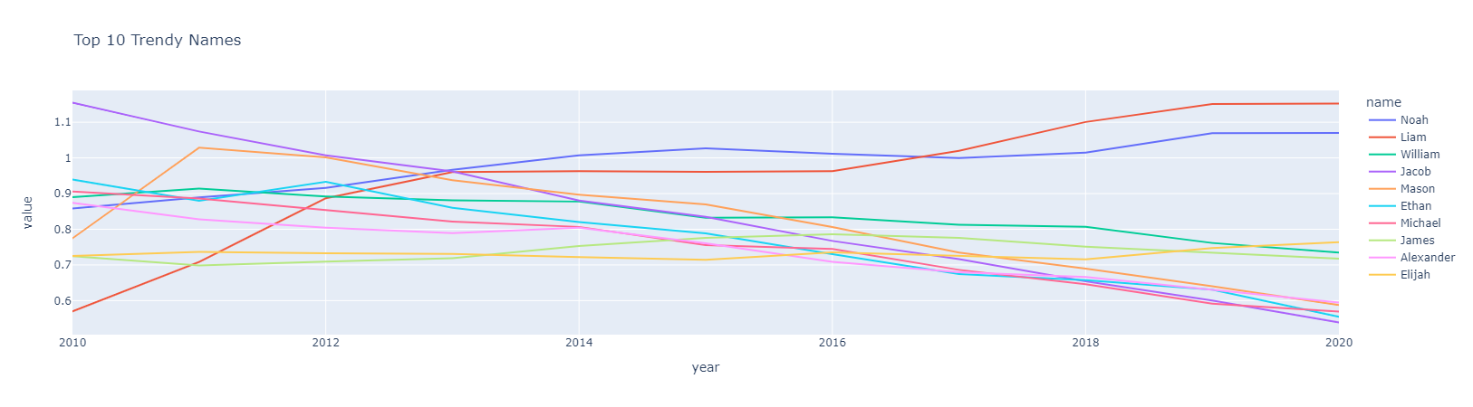 Figure 1.1 Trendy Baby Names Over Time.
Liam is still the most ‘trendy’ & popular name, according to growth, over the last 10 years.
I’m going to create another function to grab the year where the name of interest is the highest.
def when_most_births(name):

    if name in set(df_m["name"]):

        highest = df_m[df_m["name"] == name].groupby("year")["count"].sum().sort_values(ascending = False)[:1]
        in_2020 = df_m[(df_m["name"] == name) & (df_m["year"] == 2020)]["count"].sum()

        print("Name {} was most popular in {} with {} kids given this name.\n".format(name, int(highest.index[0]), highest.iloc[0]))

        print('In 2020 there were {} babies in total who were given the name {}.\n'.format(in_2020, name))

        px.line(df_m[df_m["name"] == name], x="year", y="count", color = "name", title=f"Baby Name {name} Over Time").show()

    else:
        print(f"Name {name} is not in the database.")
when_most_births("Enzo")
Name Enzo was most popular in 2020 with 2201 kids given this name.

In 2020 there were 2201 babies in total who were given the name Enzo.
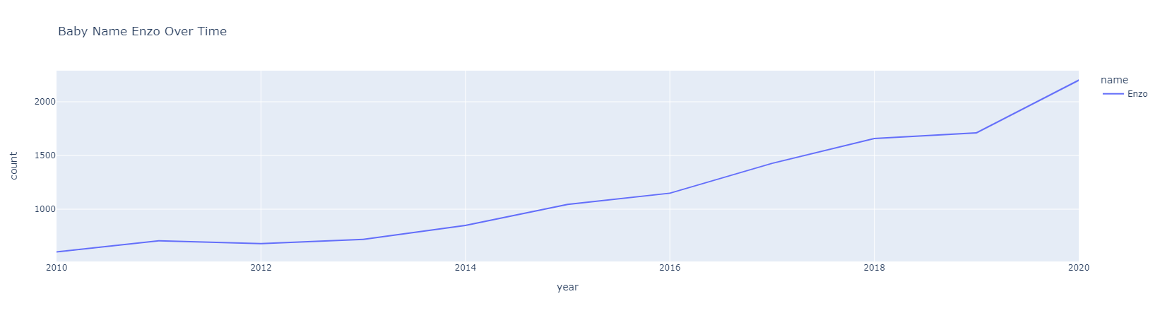 Figure 1.2 Most Popular Over Time.
Using a function from a kaggle notebooke we will
Create a metric that measure spikes & then has a drop off.
- Divide a names maximum count by its total count.
Most Sudden Names
df = df_m.groupby(['name', 'gender'])['count'].agg(['sum', 'max'])

df_ = df.reset_index()

df_['spike_fall'] = df_['max']/df_['sum']

popular = df_.sort_values(by='spike_fall',ascending=False)

popular_df = popular[popular["sum"] > 5000]
popular_df.head(5)
Lets use our function when_most_births to plot what names we want to examine for name spikes/falls.
when_most_births("Jase")
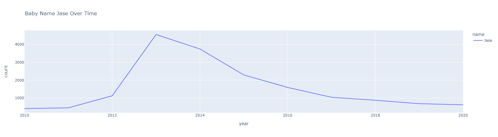 Figure 1.3 Spike-Fall Over Time.
Name Jase was most popular in 2013 with 4552 kids given this name.

In 2020 there were 624 babies in total who were given the name Jase.
Examining The Spike-Fall Names
- Jase is a great example of the spike/fall being able to capture an example of a name that peaked in 2013 and has dropped in popularity.
- For some high ranked spike/fall names we do not see the fade part because their peak year is the last one in the dataset.
As you might imagine, this is not the end of finding a baby name. Some open questions are:
- How do I actually use this data to choose a name and not just use the analysis for avoiding names?
- What if a trendy name is something we want?
Further analysis can look into both gender names to create a metric that finds the optimal gender neutral name.
We solved the initial problem of avoiding specific names but the question of interest is still left open-ended. Luckily we have 6 months remaining to decide on a name.