Altuve vs Biggio with Bayesian A/B Testing.
Who is a better batter?: Craig Biggio or Jose Altuve? Inspiration for this post comes after reading David Robinson’s post comparing Mike Piazza vs Hank Aaron using Bayesian A/B testing here. At the end of 2014 Jose Altuve has a higher career batting average (630 hits/ 2083 at-bats=.302) than Craig Biggio (3060 hits/ 10876 at-bats=.281). Can we say that Altuve’s batting skill is actually better than Biggio’s or could it be that Altuve has not played long enough to regress towards the mean? In this post we will compare two batters using an empirical Bayesian approach to batting statistics to determine who is the better batter and by how much? Understanding the difference between the two proportions is important in A/B testing. One of the most common examples of A/B testing is comparing clickthrough rates (“out of X impressions, there have been Y clicks”)- which on the surface is similar to our batting average estimation problem (“out of X at-bats, there have been Y hits”). Lets define the problem in terms of the difference between each players posterior distribution, and look at three mathematical and computational strategies we can use to solve the issue related to baseball statistics although many A/B tests can apply the same principles.
Setup
Grab career batting average of non-pitchers (allow players that have pitched <= 3 games, like Ty Cobb)
library(dplyr)
library(tidyr)
library(Lahman)
library(knitr)
library(ggplot2)
theme_set(theme_bw())

pitchers <- Pitching %>%
  group_by(playerID) %>%
  summarize(gamesPitched = sum(G)) %>%
  filter(gamesPitched > 3)

career <- Batting %>%
  filter(AB > 0) %>%
  anti_join(pitchers, by = "playerID") %>%
  group_by(playerID) %>%
  summarize(H = sum(H), AB = sum(AB)) %>%
  mutate(average = H / AB)
Add player names
career <- Master %>%
  tbl_df() %>%
  select(playerID, nameFirst, nameLast) %>%
  unite(name, nameFirst, nameLast, sep = " ") %>%
  inner_join(career, by = "playerID")
Estimate hyperparameters alpha0 and beta0 for empirical Bayes
career_filtered <- career %>% filter(AB >= 500)
m <- MASS::fitdistr(career_filtered$average, dbeta,
                    start = list(shape1 = 1, shape2 = 10))

alpha0 <- m$estimate[1]
beta0 <- m$estimate[2]
For each player, update the beta prior based on the evidence to get posterior parameters alpha1 and beta1
career_eb <- career %>%
  mutate(eb_estimate = (H + alpha0) / (AB + alpha0 + beta0)) %>%
  mutate(alpha1 = H + alpha0,
         beta1 = AB - H + beta0) %>%
  arrange(desc(eb_estimate))
So let’s take a look at the two batters in question, Craig Biggio and Jose Altuve
# Save them as separate objects too for later:
biggio <- career_eb %>% filter(name == "Craig Biggio")
altuve <- career_eb %>% filter(name == "Jose Altuve")
bagwell <- career_eb %>% filter(name == "Jeff Bagwell")
two_players <- bind_rows(biggio, altuve)

kable(head(two_players))
| Player ID | Name | H | AB | Average | eb_estimate | alpha1 | beta1 |
|---|---|---|---|---|---|---|---|
| biggicr01 | Craig Biggio | 3060 | 7816 | 0.281 | 0.281 | 3137 | 8035 |
| Jose Altuve | Jose Altuve | 1046 | 2315 | 0.311 | 0.307 | 1123 | 2534 |
We see that Altuve has slightly higher batting average, and a higher shrunken empirical bayes estimate ((H + α0)/(AB* + *α*0 + *β*0), where *α*0 and *β*0 are our priors). But is Altuve’s true probability of getting a hit higher than Biggios? Or is the difference due to chance? The answer lies in considering the range of plausible values for their “true” batting averages after we have taken their batting average (record) into account, or the “actual posterior distributions”. These posterior distributions are modeled as beta distributions with the parameters Beta(*α*0 + *H*, *α*0 + *β*0 + *H* + *AB)
library(broom)
library(ggplot2)
theme_set(theme_bw())

two_players %>%
inflate(x = seq(.26, .33, .00025)) %>%
mutate(density = dbeta(x, alpha1, beta1)) %>%
ggplot(aes(x, density, color = name)) +
geom_line() +
labs(x = "Batting average", color = "")
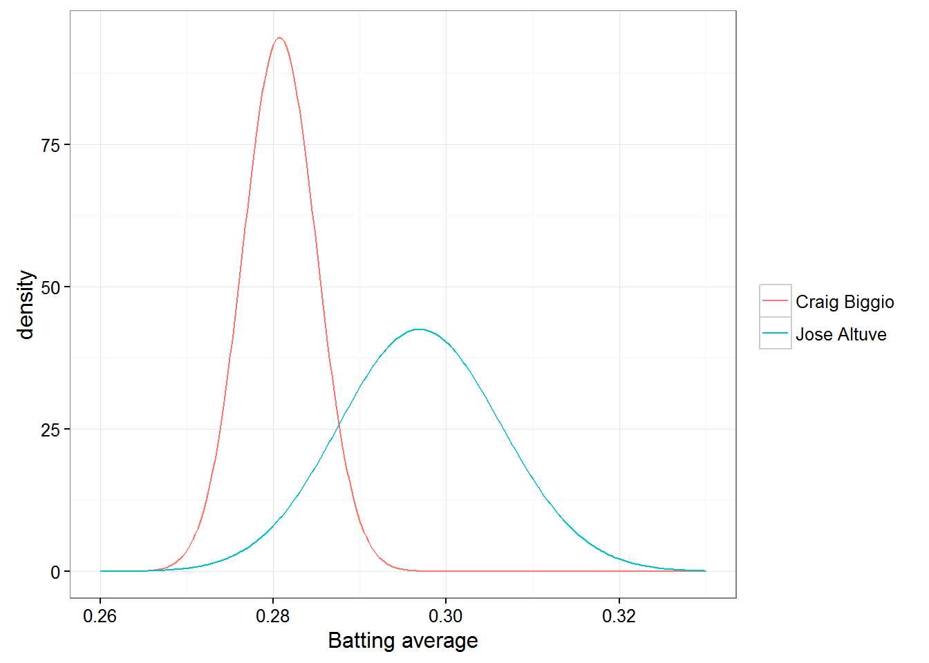
This posterior is a probalistic representations of our uncertainty in each estimate. When we ask what is the probability Altuve is better, we are asking “if I drew a random draw from Altuve’s batting record and a random draw from Biggio’s, what is the probability Altuve is higher”? Notice how Biggio’s and Atluve’s distribution overlap near the .290 range. Although by examing the distribution there is NOT enough uncertainty in each of the estimates to determine that Biggio could be a better hitter than Altuve at the current year statistics in 2014. If we took a random draw from Biggio’s distribution from Altuve’s, its very unlikely Biggio would be higher.
Lets throw Bagwell in thier to compared two retired Astro players:
career_eb %>%
filter(name %in% c("Craig Biggio", "Jose Altuve", "Jeff Bagwell")) %>%
inflate(x = seq(.26, .33, .00025)) %>%
mutate(density = dbeta(x, alpha1, beta1)) %>%
ggplot(aes(x, density, color = name)) +
geom_line() +
labs(x = "Batting average", color = "")
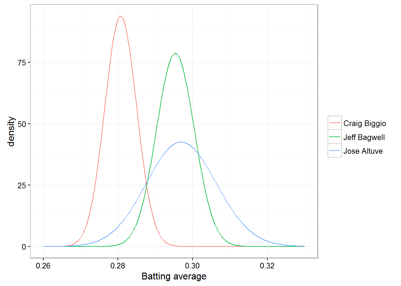
Jeff Bagwell won a Silver Slugger Award in 1994 and had an excellent batting record. Notice the vast amount of overlap in Bagwell and Altuve’s distributions. This means there is enough uncertainty in the estimates that Bagwell could easily be a better batter than Altuve.
Posterior Probability
We may be interested in the probability that Altuve is a stronger hitter than Biggio within our model. From the graph we can already tell that its greater than 50%, how can we quantify this? We need to kow the probability one beta ditribution is greater than another. I’m going to illustrate three common routes in solving a Bayesian problem:
1) Simulation of posterior draws 2) Numerical integration 3) Closed-form approximation
Simulation of posterior draws
Simulation is the quickest way around not having to do any math. Using each player’s α1 and β1 parameters, draw a million items from each of them using rbeta, and compare results:
altuve_simulation <- rbeta(1e6, altuve$alpha1, altuve$beta1)
biggio_simulation <- rbeta(1e6, biggio$alpha1, biggio$beta1)
bagwell_simulation <- rbeta(1e6, bagwell$alpha1, bagwell$beta1)
sim <- mean(altuve_simulation > biggio_simulation)
head(sim)

## [1] 0.999
sim2 <- mean(bagwell_simulation > altuve_simulation )
sim2

## [1] 0.103
A 99% probability that Altuve is a better batter than Biggio. For fun lets compare Altuve to Bagwell. A much lower probability of 10% that Bagwell is a better batter than Altuve. You could turn up or down the number of draws depending on how much you value speed vs precision. We didn’t have to do any mathematical derivation or proofs. Even if we had a more complicated model, the process for simulating from it would still straightforward. This is one of the reasons Bayesian simulation approaches have become popular: computational power has gotten cheap, while doing math is as expensive.
Integration
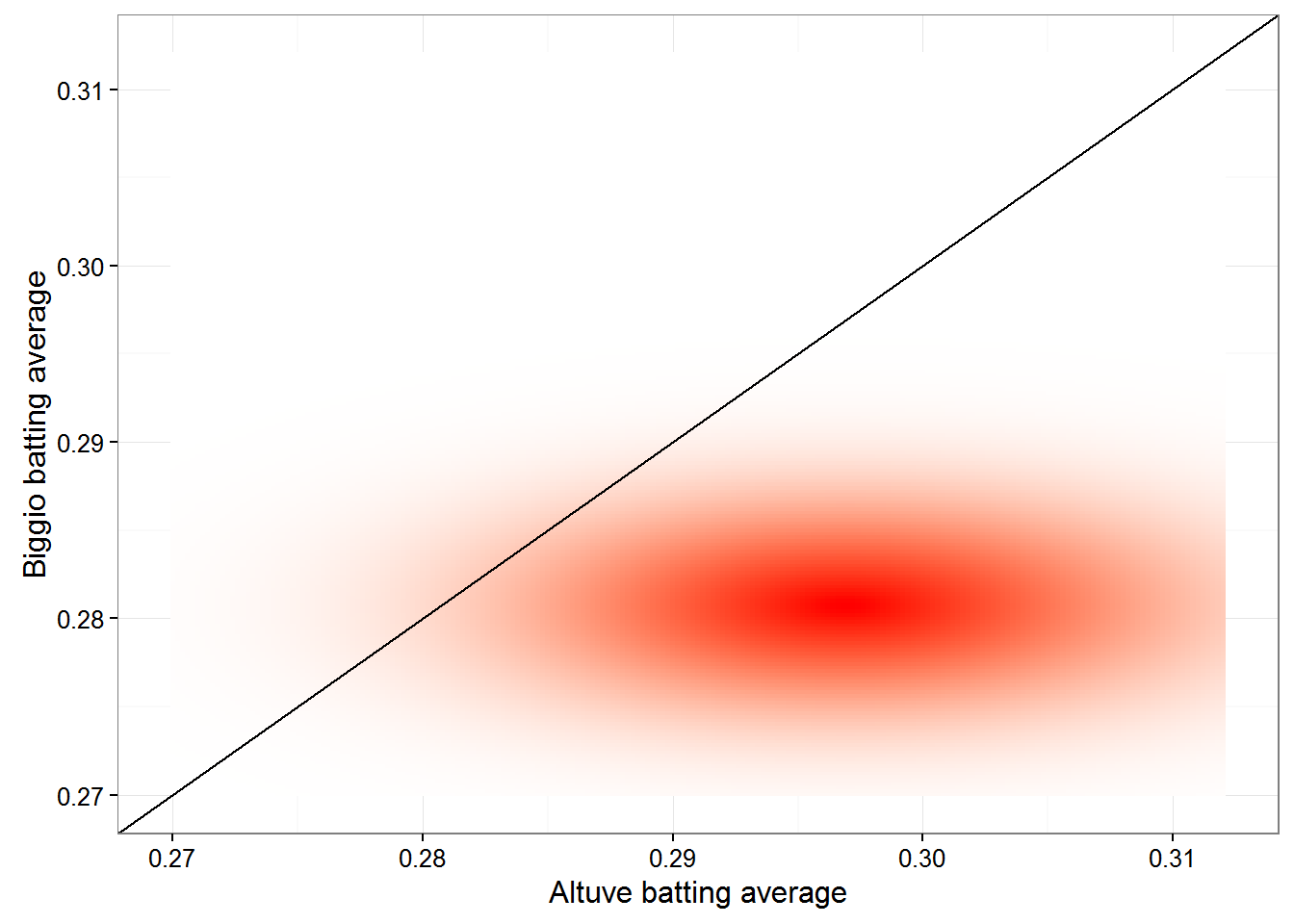
These two posteriors have their own independent distribution, and together they form a joing distribution - a density over particular pairs of x and y. The joint distribution could be imagined as a density cloud:
library(tidyr)

x <- seq(.270, .312, .0002)
crossing(altuve_x = x, biggio_x = x) %>%
mutate(altuve_density = dbeta(altuve_x, altuve$alpha1, altuve$beta1),
biggio_density = dbeta(biggio_x, biggio$alpha1, biggio$beta1),
joint = altuve_density * biggio_density) %>%
ggplot(aes(altuve_x, biggio_x, fill = joint)) +
geom_tile() +
geom_abline() +
scale_fill_gradient2(low = "white", high = "red") +
labs(x = "Altuve batting average",
y = "Biggio batting average",
fill = "Joint density") +
theme(legend.position = "none")
Here we are asking what fraction of the joint probability density lies below the black line, where altuve’s average is greater than Biggio’s. Clearly more lies below than above, confirming the posterior probability that Altuve is a better hitter by 99%. Using numerical integration to calculate this quantitatively would look like this in R:
d <- .00002
limits <- seq(.26, .33, d)
sum(outer(limits, limits, function(x, y) {
(x > y) *
dbeta(x, altuve$alpha1, altuve$beta1) *
dbeta(y, biggio$alpha1, biggio$beta1) *
d ^ 2
}))

## [1] 0.997
The approach becomes harder to control in problems that have many dimensions.
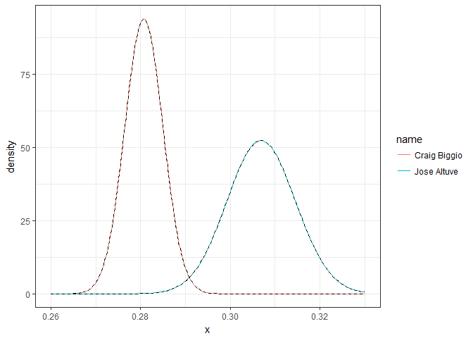
Closed-form approximation
Closed-form approximation is a much faster approximation approach. When α and β are both fairly large, the beta starts looking similar to a normal distribution, so much so that it can be closely approximated. If you draw the normal approximation to the Altuve and Biggio, they are visually indistinguishable:
two_players %>%
mutate(mu = alpha1 / (alpha1 + beta1),
var = alpha1 * beta1 / ((alpha1 + beta1) ^ 2 * (alpha1 + beta1 + 1))) %>%
inflate(x = seq(.26, .33, .00025)) %>%
mutate(density = dbeta(x, alpha1, beta1),
normal = dnorm(x, mu, sqrt(var))) %>%
ggplot(aes(x, density, group = name)) +
geom_line(aes(color = name)) +
geom_line(lty = 2)
The probability one normal is greater than another is very easy to calculate mathematically:
h_approx <- function(alpha_a, beta_a,
alpha_b, beta_b) {
u1 <- alpha_a / (alpha_a + beta_a)
u2 <- alpha_b / (alpha_b + beta_b)
var1 <- alpha_a * beta_a / ((alpha_a + beta_a) ^ 2 * (alpha_a + beta_a + 1))
var2 <- alpha_b * beta_b / ((alpha_b + beta_b) ^ 2 * (alpha_b + beta_b + 1))
pnorm(0, u2 - u1, sqrt(var1 + var2))
}

h_approx(altuve$alpha1, altuve$beta1, biggio$alpha1, biggio$beta1)

## [1] 0.999
The calculation is vecorizable in R. The downside being that for low α or low β, the normal approximation to the beta is going to fit rather poorly. The closed-form approximation is systematically biased. In certain problems it will give too high of an answer and some cases too low. When we have prior alpha and beta we are safe using the closed-form approximation.
Confidence and credible intervals
In frequentist statistics is a contigency table comparing two proporations. Such as:
| Player | Hits | Misses |
|---|---|---|
| Craig Biggio | 3060 | 7816 |
| Jose Altuve | 1046 | 2315 |
A common classical way to approach contingency table problems in with Pearson’s chi-squared test, implemented in R as prop.test:
prop.test(two_players$H, two_players$AB)

    ##
    ##  2-sample test for equality of proportions with continuity
    ##  correction
    ##
    ## data:  two_players$H out of two_players$AB
    ## X-squared = 10, df = 1, p-value = 9e-04
    ## alternative hypothesis: two.sided
    ## 95 percent confidence interval:
    ##  -0.0478 -0.0119
    ## sample estimates:
    ## prop 1 prop 2
    ##  0.281  0.311
We see a significant value less than .05. Therefore confirming our posterior distribution. Prop test also gives you a confidence interval for the difference between the two players. Now we will use empirical Bayes to compute the credible interval about the difference in Altuve and Biggio. We can do this simulation or integration but we will use our normal approximation approach:
credible_interval_approx <- function(a, b, c, d) {
u1 <- a / (a + b)
u2 <- c / (c + d)
var1 <- a * b / ((a + b) ^ 2 * (a + b + 1))
var2 <- c * d / ((c + d) ^ 2 * (c + d + 1))

mu_diff <- u2 - u1
sd_diff <- sqrt(var1 + var2)

data_frame(posterior = pnorm(0, mu_diff, sd_diff),
estimate = mu_diff,
conf.low = qnorm(.025, mu_diff, sd_diff),
conf.high = qnorm(.975, mu_diff, sd_diff))
}
credible_interval_approx(altuve$alpha1, altuve$beta1, biggio$alpha1, biggio$beta1)
## # A tibble: 1 x 4
##   posterior estimate conf.low conf.high
##       <dbl>    <dbl>    <dbl>     <dbl>
## 1     0.999  -0.0262  -0.0433  -0.00911
Now lets grab 20 random players and compare then to Altuve. We will also calculate a Confidence Interval Using prop.test
set.seed(188)

intervals <- career_eb %>%
filter(AB > 10) %>%
sample_n(20) %>%
group_by(name, H, AB) %>%
do(credible_interval_approx(altuve$alpha1, altuve$beta1, .$alpha1, .$beta1)) %>%
ungroup() %>%
mutate(name = reorder(paste0(name, " (", H, " / ", AB, ")"), -estimate))
f <- function(H, AB) broom::tidy(prop.test(c(H, altuve$H), c(AB, altuve$AB)))
prop_tests <- purrr::map2_df(intervals$H, intervals$AB, f) %>%
mutate(estimate = estimate1 - estimate2,
name = intervals$name)

all_intervals <- bind_rows(
  mutate(intervals, type = "Credible"),
  mutate(prop_tests, type = "Confidence")
)

ggplot(all_intervals, aes(x = estimate, y = name, color = type)) +
geom_point() +
geom_errorbarh(aes(xmin = conf.low, xmax = conf.high)) +
xlab("Altuve average - Player average") +
ylab("Player")
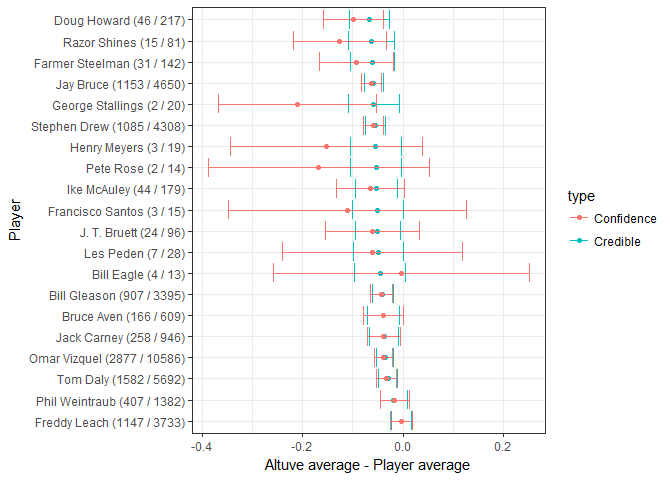
Because there is not a lot of information on certain players their credible intervals end up smaller than their confidence intervals. This is because we are able to use the prior to adjust the expectations (Esix Snead may have ended up with a higher batting average than Altuve but we are sure it was not .25 higher). When provided with a lot of information, the confidence and credible intervals approach almost perfectly. Therefore, empirical Bayes A/B credible intervals are a way to “shrink” frequentist confidence intervals, by sharing power across players.
Conclusion:
We are acting as if baseball players make up one homogeneous pool, this is mathematically convenient but its ignoring a lot of information about players. Pitchers faced, stadiums played in, length of career. For instance, ignoring how long Altuve’s career compared to Biggio’s 20 year career. This leads to bias where empirical Bayes tends to overestimate players with very few at-bats. Also, this post is ONLY comparing Altuve’s BATTING AVERAGE to Biggio’s and not taking into account how valuable Biggio was to the Astros over the years. Starting at catcher then moving to second base and even dabbling in center field. For a moving piece on Biggio read Bill James analysis of Craig Biggio here. Despite a little negativity there is one thing James hit spot on, “Biggio was the guy who would do whatever needed to be done.”